
How to calculate a weighted average in Excel, with examples


On this page
Key takeaways
- The formula is =SUMPRODUCT(values, weights) / SUM(weights). It works with percentages, credit hours, units sold or any other weight.
- AVERAGE treats every row the same, so it gives the wrong answer whenever some rows count more than others.
- If your weights are percentages that add up to 100%, SUMPRODUCT on its own gives the same result, but keeping the division protects you when the total drifts.
- To average only some rows, multiply by a condition inside SUMPRODUCT and divide by SUMIF.
- Google Sheets has AVERAGE.WEIGHTED. Excel does not, so SUMPRODUCT is the standard method there.
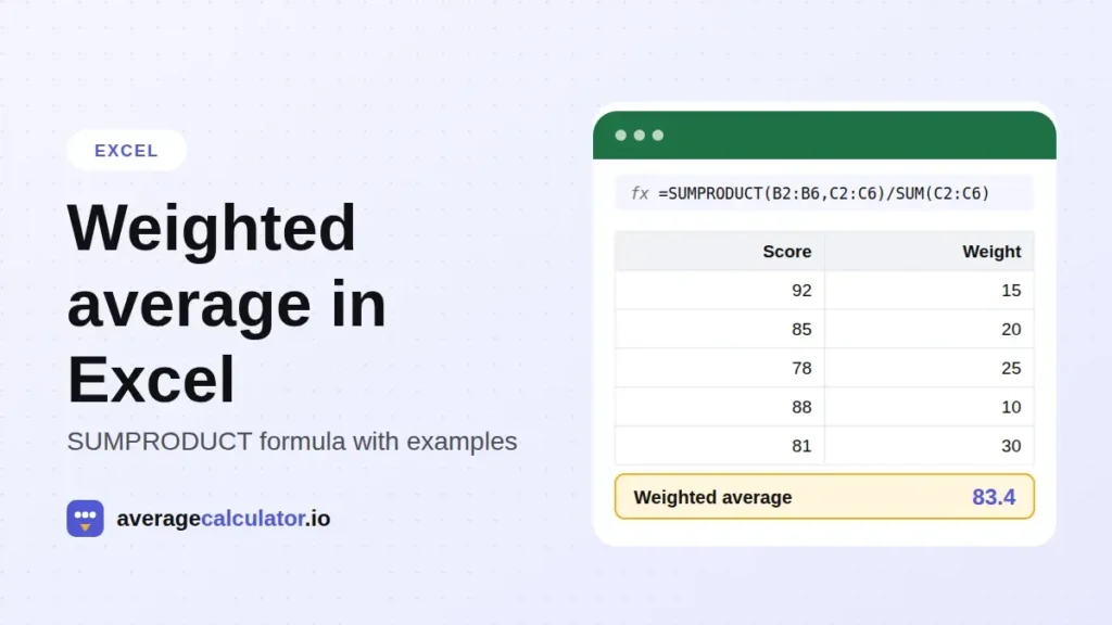
Excel has no built-in weighted average function, so you build one from two functions. SUMPRODUCT multiplies each value by its weight and adds the results. SUM adds up the weights. Divide the first by the second:
=SUMPRODUCT(B2:B6, C2:C6) / SUM(C2:C6)Put your values in B2:B6 and the weights in C2:C6, change the ranges to match your sheet, and press Enter. The same formula works whether the weights are percentages, credit hours, quantities or points.
The weighted average formula in Excel
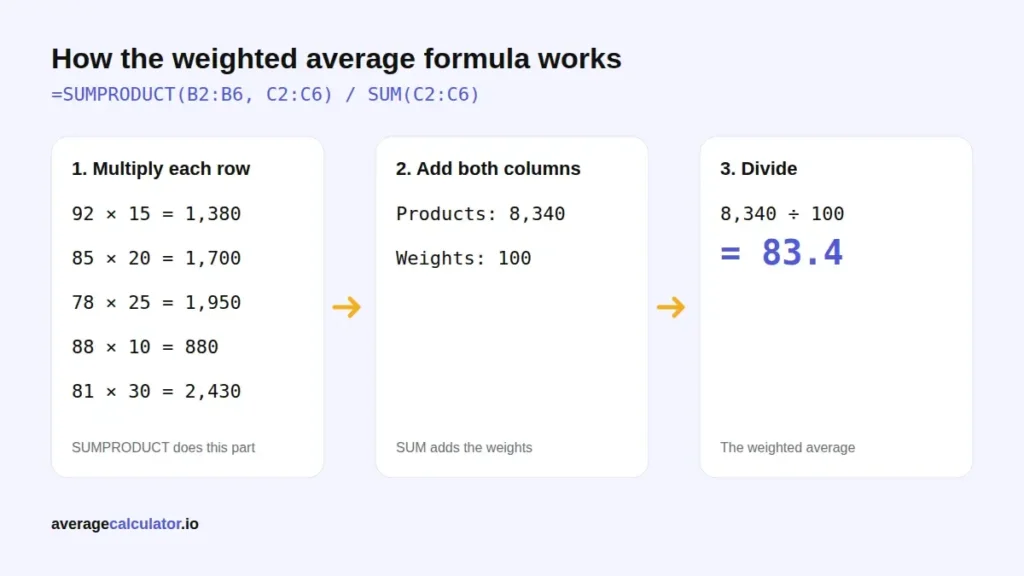
A weighted average is the sum of each value times its weight, divided by the sum of the weights. In Excel that becomes:
=SUMPRODUCT(values, weights) / SUM(weights)- SUMPRODUCT(values, weights) multiplies the first value by the first weight, the second by the second, and so on, then adds all the products.
- SUM(weights) adds the weights.
- The division scales the result back to the same units as your values.
Both ranges must be the same size and shape. They can sit in columns or in rows, as long as they line up.
Step-by-step example: a course grade
Say a course grade is made of five parts, each with its own weight:
| Component | Score | Weight (%) |
|---|---|---|
| Homework | 92 | 15 |
| Quizzes | 85 | 20 |
| Midterm | 78 | 25 |
| Project | 88 | 10 |
| Final exam | 81 | 30 |
- Type the component names in column A, the scores in B2:B6 and the weights in C2:C6.
- Click an empty cell, such as B8.
- Type =SUMPRODUCT(B2:B6, C2:C6) / SUM(C2:C6) and press Enter.
- Excel returns 83.4.
Behind the scenes, SUMPRODUCT works out 92 × 15 + 85 × 20 + 78 × 25 + 88 × 10 + 81 × 30 = 8,340. SUM adds the weights to get 100. And 8,340 / 100 = 83.4.
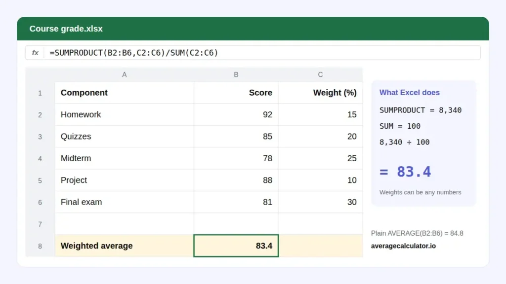
For comparison, =AVERAGE(B2:B6) returns 84.8. The plain average is higher because the two lowest scores, the midterm and the final exam, carry more than half of the total weight.
Why AVERAGE gives the wrong answer
AVERAGE adds the values and divides by how many there are. It has no way to know that the final exam counts twice as much as the homework. Any time your rows are not equally important, such as graded work, orders of different sizes or survey groups of different sizes, AVERAGE will be off by however much the weights would have pulled the result.
The gap can be large. With weights heavily tilted toward one row, the plain average can miss the weighted one by several points, which is the difference between a B and a C on a transcript.
When the weights are percentages that add up to 100%
If you type the weights as 15%, 20%, 25%, 10% and 30%, Excel stores them as 0.15, 0.2 and so on, and SUM(C2:C6) returns 1. Dividing by 1 changes nothing, so this shorter formula gives the same 83.4:
=SUMPRODUCT(B2:B6, C2:C6)Keep the full formula anyway. If someone edits a weight and the total becomes 95%, the short version quietly returns a wrong number, while the version with / SUM(C2:C6) still gives the correct weighted average for the weights that are there.
Do not mix the two styles in one column. A weight of 15 next to a weight of 20% makes Excel treat one as fifteen and the other as a fifth, and the result will be far off.
Weighted average price in Excel
The same formula gives the average price per unit when you bought or sold different quantities at different prices. Here the price is the value and the number of units is the weight:
| Region (A) | Price per unit (B) | Units (C) |
|---|---|---|
| East | $12.50 | 400 |
| West | $13.20 | 150 |
| East | $11.80 | 600 |
| West | $12.90 | 250 |
| East | $12.10 | 300 |
=SUMPRODUCT(B2:B6, C2:C6) / SUM(C2:C6)The result is $12.30 per unit: $20,915 in total across 1,700 units. A plain AVERAGE of the five prices gives $12.50, which overstates the cost because the largest order, 600 units, was also the cheapest.
Weighted average with a condition
To get the weighted average price for the East region only, add a condition inside SUMPRODUCT and swap SUM for SUMIF:
=SUMPRODUCT((A2:A6="East") * B2:B6 * C2:C6) / SUMIF(A2:A6, "East", C2:C6)(A2:A6=”East”) returns TRUE or FALSE for each row. Multiplying turns those into 1 and 0, so only the East rows add to the total. SUMIF adds the East units, 1,300. The result is $12.08.
For two conditions, such as region and quarter, multiply both tests and use SUMIFS:
=SUMPRODUCT((A2:A6="East") * (D2:D6="Q1") * B2:B6 * C2:C6) / SUMIFS(C2:C6, A2:A6, "East", D2:D6, "Q1")Other ways to write it
- In Excel 365 and Excel 2021, =SUM(B2:B6 * C2:C6) / SUM(C2:C6) also works and gives the same result. Older versions need Ctrl+Shift+Enter for this form, so SUMPRODUCT is the safer choice if others will open the file.
- For a handful of rows you can write it out by hand: =(B2*C2 + B3*C3 + B4*C4) / SUM(C2:C4). It is easy to read, but easy to break when you add a row.
- Google Sheets has a built-in function: =AVERAGE.WEIGHTED(B2:B6, C2:C6). The SUMPRODUCT formula works there too.
Common errors and how to fix them
#VALUE!
The two ranges are different sizes, for example B2:B6 and C2:C7. SUMPRODUCT needs them to match exactly.
#DIV/0!
The weights add up to zero, usually because the weight cells are empty. Fill them in or point SUM at the right range.
A result that is too low
A blank score next to a weight counts as zero and drags the average down. If a score is not in yet, leave the weight blank as well, or remove the row. Numbers stored as text also count as zero inside SUMPRODUCT. Look for small green triangles in the cells and convert them with Convert to Number.
A result that is far too big or too small
Some weights are typed as whole numbers (15) and others as percentages (15%). Pick one style for the whole column.
Check your answer
Copy the two columns from your sheet and paste them into the weighted average calculator. It shows the same result with every multiplication and the final division written out, so you can see which row is off if your spreadsheet disagrees. For percentages that come from different totals, the average percentage calculator does the weighting for you.
Frequently asked questions
What is the formula for a weighted average in Excel?
=SUMPRODUCT(values, weights) / SUM(weights). For scores in B2:B6 and weights in C2:C6, that is =SUMPRODUCT(B2:B6, C2:C6) / SUM(C2:C6).
Does Excel have a weighted average function?
No. Excel has no WEIGHTED.AVERAGE or AVERAGE.WEIGHTED function, so you combine SUMPRODUCT and SUM. Google Sheets does have AVERAGE.WEIGHTED.
Do the weights need to add up to 100%?
No. Dividing by SUM(weights) handles any total. Credit hours of 3, 4 and 3 work the same way as percentages.
How do I calculate a weighted average with percentages in Excel?
Enter the weights as percentages, such as 15% and 20%, and use the same formula. If the percentages add up to exactly 100%, =SUMPRODUCT(values, weights) alone gives the answer.
How do I calculate a weighted average in Excel with criteria?
Multiply by the condition inside SUMPRODUCT and divide with SUMIF, for example =SUMPRODUCT((A2:A6=”East”) * B2:B6 * C2:C6) / SUMIF(A2:A6, “East”, C2:C6).
Why is my weighted average wrong in Excel?
The usual causes are ranges of different sizes, blank scores that have a weight, numbers stored as text, and a weight column that mixes whole numbers with percentages.
How do I calculate a weighted average in Google Sheets?
Use =AVERAGE.WEIGHTED(values, weights), or the same SUMPRODUCT formula you would use in Excel.
About the author
More from the blog

Spotted a mistake in this article? Tell us the numbers you used and what you expected, and we will check it.
Report an error