
Degrees of freedom calculator
Work out the degrees of freedom for twelve statistical tests, from a one-sample t-test to two-way ANOVA, and get the critical value that goes with them.

 By Michael O'Brien · Reviewed by Paul Lewis✓ Fact-checked
Enter your sample sizes
How to use the degrees of freedom calculator
- 1Pick your test
Twelve tests are covered, from a one-sample t-test to two-way ANOVA and multiple regression. The fields change to match.
- 2Enter sample sizes, or paste the data
If you already know n, type it. If you have the numbers, switch to Raw data and the calculator counts them and works out the variances for you.
- 3Choose a significance level
0.05 is the usual choice. It decides the critical value you compare your test statistic against.
- 4Read the df and the critical value
You get the degrees of freedom, the formula with your numbers in it, the critical value, and a slice of the distribution table around your df.
Step-by-step solution
What are degrees of freedom?
Degrees of freedom is the count of values in a calculation that are still free to vary. The University of Texas Statistical Online Services puts it as the number of values which are free to vary, and the seat analogy they use makes it concrete: in a room with 30 chairs, 29 people can sit wherever they like, and the last person has no choice left.
The same thing happens once you estimate something from your data. Say five numbers have a mean of 20, so they add up to 100. You can set the first four to anything at all, say 14, 22, 31 and 18. Those add to 85, so the fifth number has to be 15. Four values were free, one was forced, and the degrees of freedom is 4.
That is the rule behind every formula on this page. Start with how many numbers you have, then subtract one for each quantity you estimated from those same numbers. In statistics output it is nearly always written df, and occasionally as the Greek letter nu. So df in statistics and degrees of freedom mean the same thing.
Degrees of freedom formula
For a single sample the formula is:
df = n − 1
n is the number of observations, and the 1 is the sample mean, which you had to work out before you could measure anything about spread. This is the same n − 1 that appears in the denominator of the sample variance, which is why our variance calculator divides by n − 1 for a sample and by N for a population.
Every other test follows the same pattern with a different count of estimates. A two-sample t-test estimates two means, so it costs two:
df = n1 + n2 − 2
A contingency table fixes its row and column totals, so the last row and last column are forced:
df = (r − 1)(c − 1)
How to find degrees of freedom
Three questions get you there for any test:
- Count the values you actually have. For a paired test that means pairs, not measurements. For ANOVA it means every observation across all groups.
- Count what the test estimates from those same values. A t-test estimates means. A regression estimates a slope for each predictor plus an intercept.
- Subtract the second number from the first.
Worked example
You are comparing test scores for two classes. Class A has 12 students, class B has 15, and you are willing to assume the two groups have similar spread, so you run a pooled two-sample t-test.
- Total observations: 12 + 15 = 27
- Estimates: two group means
- Degrees of freedom: 27 − 2 = 25
Look 25 df up in a t table at the 0.05 level, two-tailed, and the critical value is 2.0595. If your t statistic comes out beyond ±2.0595 the difference is significant at that level. Select the same test in the calculator above and you get the df, the critical value and a slice of the t table around 25 df without opening a textbook.
Degrees of freedom for a t-test
Which formula you need depends on how many samples you have and what you are assuming about their variances.
- One-sample or paired t-test: df = n − 1. For the paired version, n is the number of pairs. Twelve people measured before and after gives n = 12, not 24.
- Two-sample t-test with equal variances: df = n1 + n2 − 2. This is the pooled test, and it assumes both groups share one variance.
- Two-sample t-test with unequal variances: the Welch-Satterthwaite formula, which mixes the two sample sizes and the two variances.
The Welch formula
df = (s1²/n1 + s2²/n2)² / [ (s1²/n1)²/(n1−1) + (s2²/n2)²/(n2−1) ]
Take the two classes again, but now class A has a standard deviation of 8.60 and class B has 16.03. The pooled formula would still say 25 df. Welch gives 22.22, because the wider spread in the larger group costs you precision.
That decimal is not a mistake. R, SPSS and Excel all use the exact value. Penn State’s STAT 415 notes say to take the integer portion when you are reading a printed table, so 22.22 becomes 22. The critical value barely moves either way: 2.0727 at 22.22 df against 2.0739 at 22.
Degrees of freedom for a chi-square test
Chi-square has two common tests and they use different formulas.
For a test of independence on a contingency table, df = (r − 1)(c − 1). A 3 by 4 table has 2 × 3 = 6 degrees of freedom. The row and column totals come from the data, so once you fill in a 2 by 3 block of cells the rest of the table is determined.
For a goodness of fit test, df = k − 1 − m, where k is the number of categories and m is how many parameters you estimated from the same data. Comparing six dice faces against an even distribution gives df = 6 − 1 = 5, because you estimated nothing. Fitting a Poisson distribution to six categories means estimating the rate from your data first, so m = 1 and df drops to 4.
People forget the m term more than anything else on this page. Skip it and your df is too high, your critical value is too big, and you end up failing to reject a null hypothesis you should have rejected.
Degrees of freedom in ANOVA and F tests
An F test uses two degrees of freedom, one for the numerator and one for the denominator, and you need both to read the table.
One-way ANOVA with k groups and N observations in total:
- Between groups (the numerator): df = k − 1
- Within groups (the denominator): df = N − k
- Total: df = N − 1
Forty students split across four teaching methods gives 3 and 36. At the 0.05 level the critical value of F(3, 36) is 2.8663. The two parts always add back to N − 1, which is a quick way to check you have not miscounted, and the sums of squares they divide into split the same way.
Two-way ANOVA splits the same total further. With a levels of factor A, b levels of factor B and n observations per cell, you get a − 1 for factor A, b − 1 for factor B, (a − 1)(b − 1) for the interaction, and ab(n − 1) for the error term. All three F tests share that error df as their denominator.
An F test comparing two variances is simpler: df1 = n1 − 1 and df2 = n2 − 1, with the larger variance on top. F tables are one-tailed, so for a two-sided test at 0.05 you look up 0.025.
Degrees of freedom in regression and correlation
A straight line through your data estimates two things, a slope and an intercept, so simple linear regression leaves df = n − 2. Thirty observations gives 28 df, and a t test on the slope uses a critical value of 2.0484 at the 0.05 level. An exponential regression fitted by taking logs carries the same n – 2, because underneath it is still a straight line with two parameters.
Add predictors and each one costs another degree of freedom. With p predictors plus an intercept, the residual df is n − p − 1. Sixty observations and four predictors leaves 55. The overall F test for that model is F(4, 55), while a t test on any single coefficient uses the 55.
This is why a model with too many predictors for its sample size stops being testable. Fit ten predictors to twelve observations and you are down to a single residual df, which makes every standard error enormous and every coefficient insignificant.
Testing a Pearson correlation uses df = n − 2 for the same reason, since r depends on both the x mean and the y mean.
Degrees of freedom table by test
Every formula the calculator uses, in one place.
| Test | Formula | Distribution |
|---|---|---|
| One-sample or paired t-test | n − 1 | t |
| Two-sample t-test, equal variances | n1 + n2 − 2 | t |
| Two-sample t-test, Welch | Welch-Satterthwaite | t |
| Chi-square independence | (r − 1)(c − 1) | Chi-square |
| Chi-square goodness of fit | k − 1 − m | Chi-square |
| One-way ANOVA | k − 1 and N − k | F |
| Two-way ANOVA | a − 1, b − 1, (a − 1)(b − 1), ab(n − 1) | F |
| F test for two variances | n1 − 1 and n2 − 1 | F |
| Simple linear regression | n − 2 | t, or F(1, n − 2) |
| Multiple linear regression | p and n − p − 1 | F |
| Pearson correlation | n − 2 | t |
The calculator prints the critical values alongside the df, which is the part a printed table makes you look up separately.
Why degrees of freedom change your answer
Degrees of freedom pick which row of the table you read, and with small samples that row matters a lot. At the 0.05 level, two-tailed, the critical t value is:
- 5 df: 2.5706
- 10 df: 2.2281
- 30 df: 2.0423
- 100 df: 1.9840
- 1,000 df: 1.9623
With 5 df your test statistic has to reach 2.5706 to count as significant. With 100 df, 1.9840 is enough. Small samples have fatter tails because a variance estimated from five numbers is itself unreliable, and the t distribution widens to account for that. Past about 120 df the difference stops mattering and t is close enough to the normal distribution’s 1.96.
Getting the df wrong by one or two is usually harmless with a large sample and can flip the conclusion with a small one. The gap between 5 and 6 df at the 0.05 level is about 0.13, which is enough to decide a borderline test.
Why use this degrees of freedom calculator?
What you get with this free degrees of freedom calculator:
- Twelve tests, including two-way ANOVA, multiple regression and the F test for two variances, which most df calculators leave out.
- The critical value at your significance level, printed next to the df instead of sent to a separate table.
- A slice of the t, chi-square or F table around your df, with your row and column highlighted.
- A plot of the distribution with the rejection region shaded, so you can see what the number is for.
- Raw data input. Paste your numbers and the calculator counts them, works out the standard deviations and runs the Welch formula for you.
- The full working, with your own numbers substituted into the formula.
- Free to use
- No sign-up
- 12 tests covered
- Critical values included
- Step-by-step working
Frequently asked questions
How do you calculate degrees of freedom?
Count your observations, then subtract one for each quantity the test estimates from the same data. For a single sample that is df = n − 1. For a two-sample t-test it is n1 + n2 − 2, because two means are estimated.
What does df mean in statistics?
df is the standard abbreviation for degrees of freedom. When software reports t(25) = 2.31, the 25 is the df, and it tells you which row of the t distribution the p-value came from.
Can you explain degrees of freedom in a simple way?
If five numbers have to average 20, you can pick any values you like for the first four. The fifth is then fixed, because the total has to come to 100. Four values were free to vary, so there are 4 degrees of freedom.
Why is it n minus 1 and not n?
Because the sample mean was worked out from the same data. Once the mean is fixed, the last value is no longer free. Dividing by n − 1 also stops the sample variance from underestimating the population variance.
How do I find degrees of freedom for a chi-square test?
For a test of independence, multiply (rows − 1) by (columns − 1). A 3 by 4 table gives 6. For a goodness of fit test, use k − 1 − m, where k is the number of categories and m is how many parameters you estimated from the data.
Can degrees of freedom be a decimal?
Yes, with Welch’s t-test. The Welch-Satterthwaite formula almost never lands on a whole number, and 22.22 df is a normal result. Statistical software uses the exact value; round down if you are reading a printed table.
Why does an F test have two degrees of freedom?
An F statistic is a ratio of two variances, and each one has its own df. The numerator df comes from the effect you are testing, the denominator df from the error term. You need both to find the right cell in an F table.
What happens if I use the wrong degrees of freedom?
You read the wrong critical value, so your p-value is wrong. Too many df gives a critical value that is too small and makes weak results look significant. Too few does the opposite. With large samples the error is often tiny; with fewer than 30 observations it can change the conclusion.
Explore our other calculators
 Average calculator
 Average percentage calculator
 Average time calculator
 Exponential Regression Calculator
 Five Number Summary Calculator
 Histogram maker
 IQR calculator
 Linear regression calculator
 Mean, Median, Mode and Range Calculator
 Outlier Calculator
 Pie Chart Maker
 Probability Calculator
 Standard deviation calculator
 Sum of Squares Calculator
 Variance calculator
 Weighted average calculator
Our latest blogs
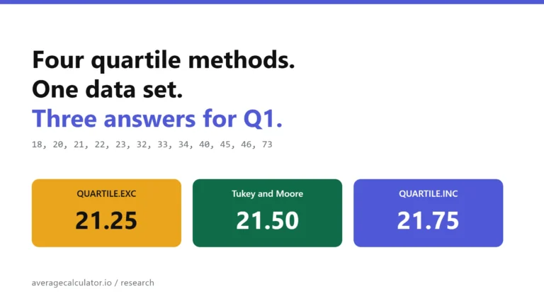
Four quartile methods, one data set, three answers for Q1
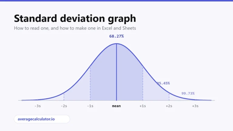
Standard deviation graph: how to read one and how to make one

Excel vs Google Sheets vs LibreOffice: how average functions handle blanks, zeros and text
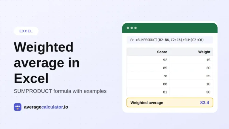
How to calculate a weighted average in Excel, with examples
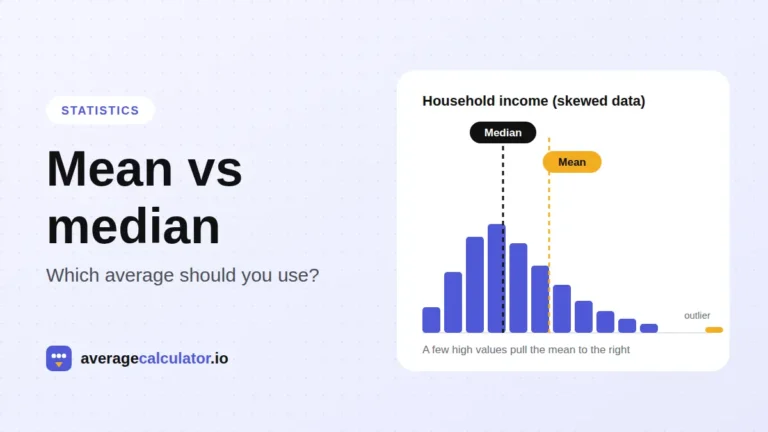
Mean vs median: which average should you use?
Who made this calculator
Spotted a mistake in this calculator? Tell us the numbers you used and what you expected, and we will check it.
Report an error