Exponential regression calculator

What exponential regression does

Exponential regression fits a curve where y multiplies by the same factor every time x goes up by one. Bacteria that increase by 37% an hour, a balance that earns 7.65% a year, a drug concentration that drops by 13% an hour: all three are the same shape, and all three are badly described by a straight line.

A straight line adds a fixed amount per step. An exponential curve multiplies by a fixed amount per step. That is the whole difference, and it is why the gap between the two grows so fast. Fit a line to seven hours of bacterial growth and the predicted count for hour nine will be far too low, because the line has no way to accelerate.

The calculator above takes x and y pairs, returns the equation in both common forms, and tells you the one thing most exponential regression tools leave out: how fast the quantity is actually growing, and how long it takes to double.

The exponential regression equation, in both forms

Two notations are in circulation and they describe exactly the same curve.

y = ab^x
y = ae^kx, where k = ln b

In both, a is the value of y when x is zero, the starting level. In the first form b is the multiplier per step: b = 1.3708 means y is 1.3708 times bigger each time x increases by one, so growth is 37.08% per step. In the second form k is the continuous rate. A positive k means growth, a negative k means decay, and k = 0 would be a flat line.

Which one you need depends on where the question came from. A TI-84 returns ab^x. Most calculus and physics courses want ae^kx because k is what appears in the differential equation. The calculator prints both, so you can copy whichever your marker is expecting.

One thing to watch: b and k are not interchangeable as percentages. A b of 1.3708 is 37.08% growth per step, but k is 0.3154, which is 31.54%. The second number is the rate compounded continuously rather than once per step. Quoting k as the growth rate is one of the more common errors in written answers.

How exponential regression is calculated

There is no separate exponential formula to memorise. Every calculator on this page, and every graphing calculator you will meet, does the same trick: take the natural log of y, then run an ordinary linear regression on x against ln y.

It works because taking logs turns multiplication into addition. If y = ab^x then ln y = ln a + x ln b, which is a straight line with intercept ln a and slope ln b. Fit that line, undo the logs, and the curve comes back.

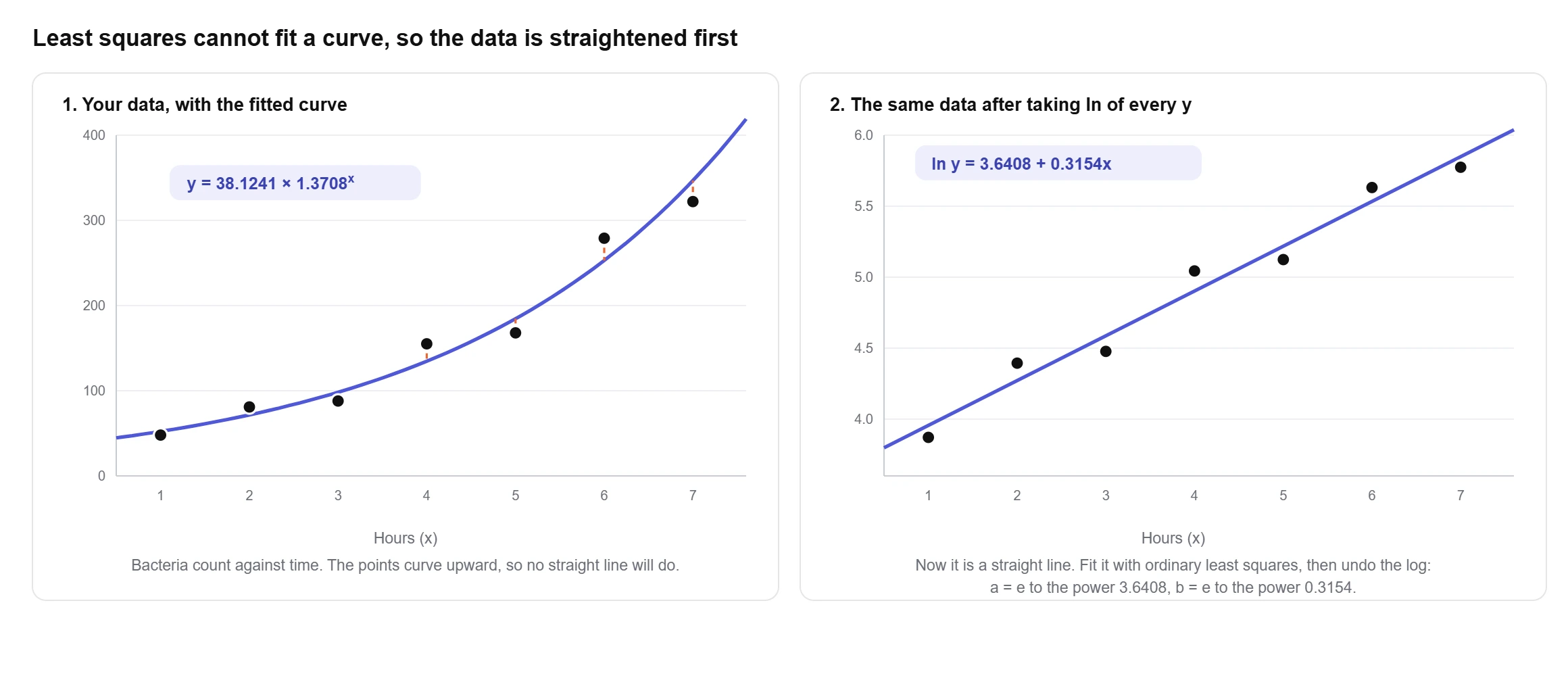
Here is the whole calculation on the bacteria sample built into the tool: hours 1 to 7 against counts of 48, 81, 88, 155, 168, 279 and 322.

Take logs first. The seven ln y values are 3.8712, 4.3944, 4.4773, 5.0434, 5.1240, 5.6312 and 5.7746. Mean x is 4 and mean ln y is 4.9023.

Now the usual least squares sums, but on ln y instead of y. Multiply each x deviation by its ln y deviation and add: 3.0933 + 1.0157 + 0.4250 + 0 + 0.2217 + 1.4578 + 2.6167 = 8.8302. The squared x deviations add to 28.

slope of the log fit: B = 8.8302 ÷ 28 = 0.3154
intercept of the log fit: A = 4.9023 − 0.3154 × 4 = 3.6408
a = e^A = 38.1241   b = e^B = 1.3708
y = 38.1241 × 1.3708^x, or y = 38.1241 e^0.3154x

That is the complete method. The only step people get wrong is the last one: A and B are the log-space answers, and they have to be exponentiated. Reporting y = 3.6408 × 0.3154^x is a fit to the logs, not to the data.

Growth rate and doubling time

An equation with a and b in it is hard to argue with in a report. A doubling time is not. Once you have b, two short conversions turn the fit into something a reader can act on.

growth per step = (b − 1) × 100%
doubling time = ln 2 ÷ k
half-life = ln 0.5 ÷ k  (when k is negative)

On the bacteria fit, b = 1.3708 gives 37.08% growth per hour and ln 2 ÷ 0.3154 = 2.1979 hours to double. The savings sample in the tool grows at 7.65% a year and doubles in 9.4013 years. The caffeine sample has k = −0.1430, so it decays 13.33% an hour with a half-life of 4.8462 hours.

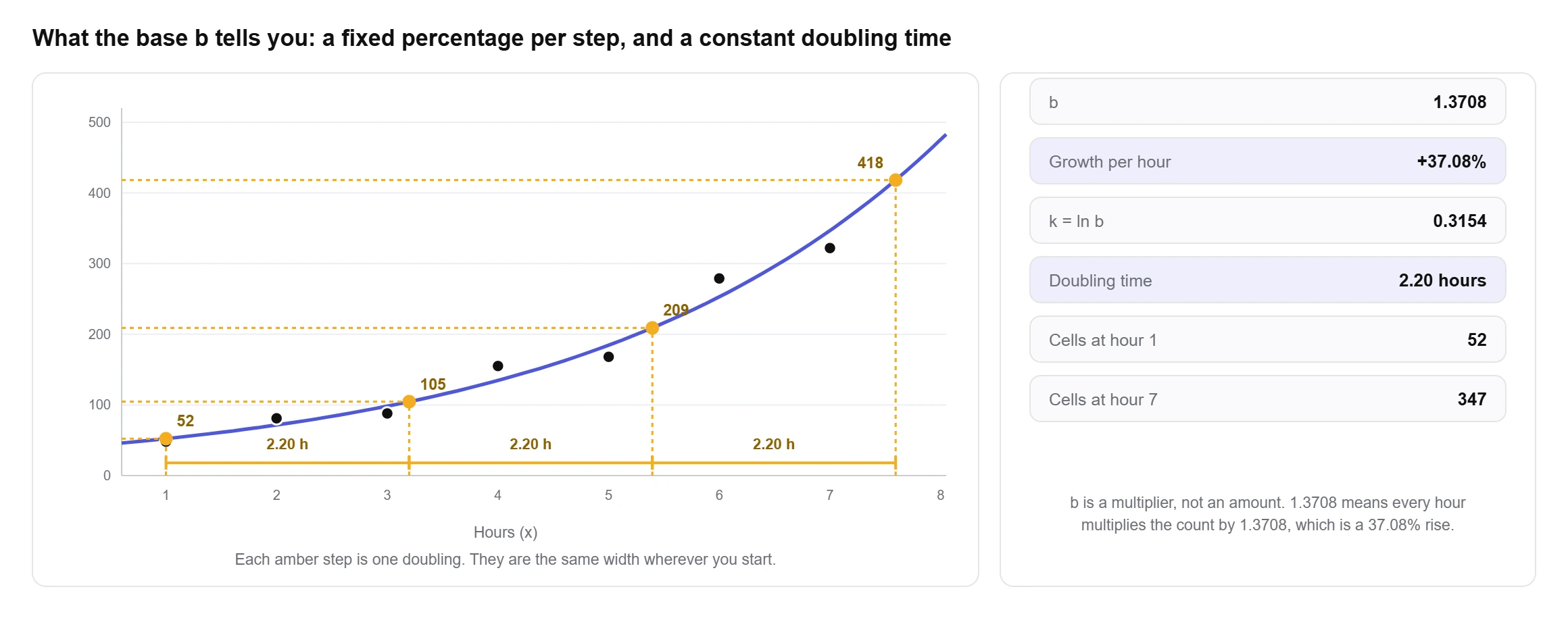
The rule of 72, dividing 72 by the percentage growth, is a decent shortcut at low rates and a bad one at high rates. At 7% it gives 10.2857 periods against a true 10.2448. At 3% it gives 24 against 23.4498. At the bacteria rate of 37.08% it gives 1.9420 hours against a true 2.1979, an error of 13%. Use it for interest rates, not for outbreaks.

Constant doubling time is also the reason semi-log plots are so common in engineering and epidemiology. Gordon Moore’s 1965 article in Electronics, the one the whole industry still quotes, made its case with component counts plotted on a log scale precisely so that a constant doubling rate would read as a straight line (Moore, Cramming more components onto integrated circuits, Electronics 38(8), 19 April 1965, pp. 114 ff).

The R squared most tools report is not the one you think

Because the fit happens in log space, there are two different R squared values available, and almost every exponential regression tool reports one of them without saying which.

The linearised R squared measures how well the straight line fits ln y. The original scale R squared measures how well the curve fits your actual y values, using the ordinary sum of squares definition: 1 minus SSE divided by SST, with both computed on y rather than ln y.

On well behaved data the two barely differ. On the bacteria sample they are 0.9727 and 0.9660. On data that is not really exponential they come apart completely. Take x = 1 to 8 against y = 3.1, 12.4, 27.9, 49.5, 78, 112, 152, 199, which is the fourth sample in the tool. The exponential fit scores 0.9190 in log space and 0.6482 against the original numbers. A tool that prints 0.9190 and calls it R squared has told you the curve explains 92% of the variation. It explains 65%.

The gap opens up because logs squash the large values. A 30 unit miss at y = 200 barely registers on a log axis, while the same miss at y = 3 is enormous. When the two numbers disagree by more than a few hundredths, that is the data telling you the curve is wrong at one end. The calculator prints both and labels them, so the disagreement is visible instead of hidden.

Exponential, power or logarithmic

Three curves get confused with each other constantly, and the confusion is understandable because all three are fitted by the same log trick with different things logged.

exponential y = ab^x   fit ln y against x
power y = ax^b   fit ln y against ln x
logarithmic y = a + b ln x   fit y against ln x

The difference in behaviour is what matters. Exponential growth has a constant doubling time and eventually beats every power curve. A power curve with b = 2 doubles when x doubles, which is much slower. A logarithmic curve flattens out and keeps rising, but by less and less.

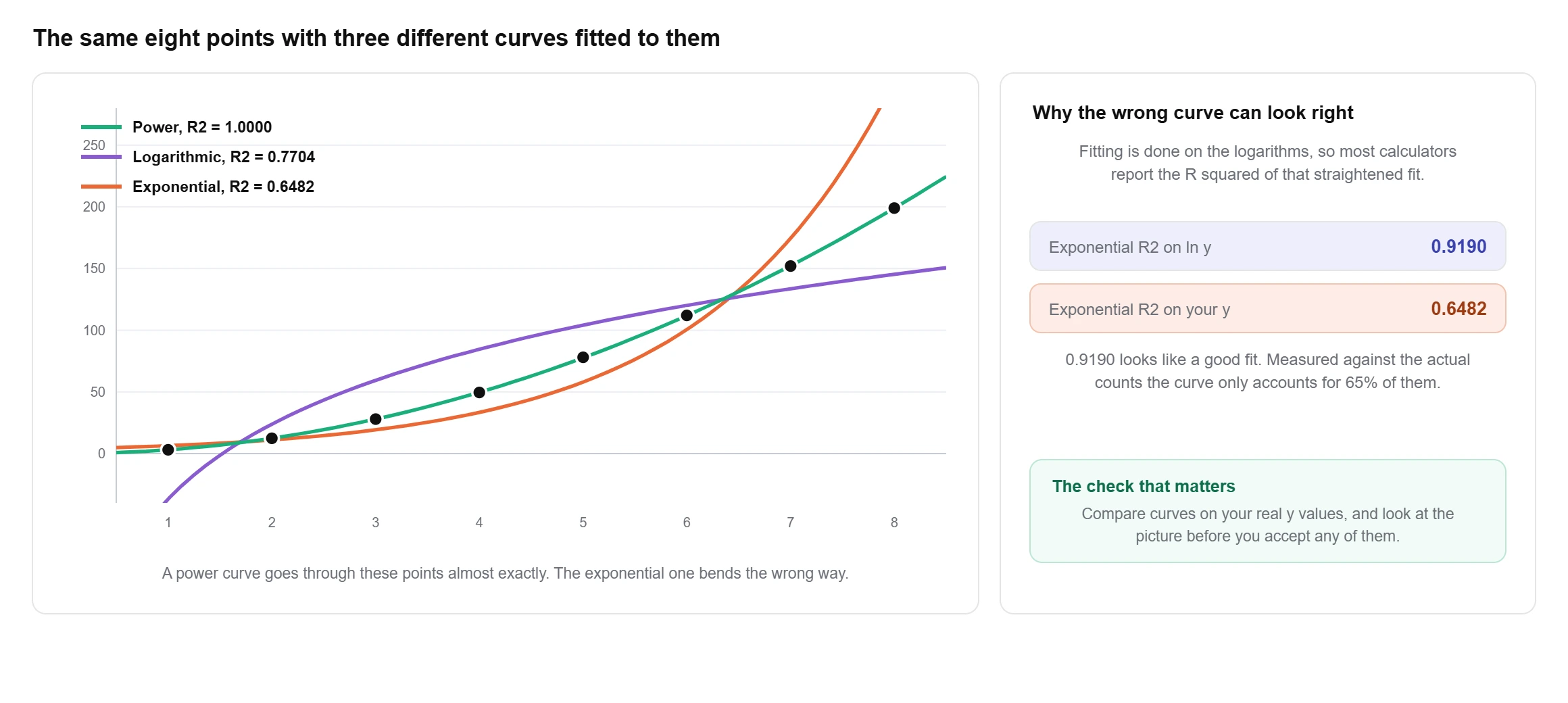
Run those eight points through all three and the ranking is not close. The power fit gives y = 3.0973x^2.0017 with an error sum of squares of 0.2597 and an R squared of 0.999992, which a four decimal display would round to a flat 1.0000. The logarithmic fit leaves 7,920.05. The exponential fit leaves 12,135.33 against a total sum of squares of 34,496.38. The data was a squared relationship all along, which the exponent of 2.0017 gives away.

Switch the calculator to Compare and it fits all three, ranks them by R squared on the original scale, and draws them on one chart. It takes one click and it is the fastest way to find out that you picked the wrong family before you write the fit into a report.

What fitting on logs quietly assumes

Least squares on ln y does not minimise the vertical gaps you see on the chart. It minimises the gaps in log space, which means it is minimising proportional error rather than absolute error. A 10% miss counts the same at y = 5 as it does at y = 5,000.

Often that is exactly right. Counts, populations and concentrations usually scatter proportionally, so the spread grows with the level. When that is true, the log fit is the better estimator. When the noise is a constant size regardless of level, it is not, and nonlinear least squares fitted directly to y is the correct method. Xiao, White, Hooten and Durham tested both on simulated and real data and found the choice depends on which error structure the measurements actually have: log transformation wins with multiplicative lognormal error, direct nonlinear regression wins with additive normal error (Ecology 92(10), 2011, pp. 1887 to 1894).

Two practical consequences follow. Zero and negative y values cannot be logged at all, so they have to be dropped or the model changed; the calculator flags them rather than silently ignoring them. And the fitted curve will usually sit slightly below the large values, because the log fit was never weighting them heavily in the first place. If the big values are the ones you care about, check the residuals at that end before trusting the prediction.

Exponential regression in Excel and Google Sheets

There are three routes, and they disagree about letters rather than about maths.

• LOGEST. Microsoft documents it as fitting y = b*m^x and returning the array {m,b}. Note the order and the naming: m is the base, the thing this page calls b, and Excel’s b is the starting value, the thing this page calls a. Enter =LOGEST(B2:B8,A2:A8) and read the first cell as the multiplier. Add ,TRUE,TRUE for the standard errors, r squared, F and the sums of squares.
• Chart trendline. Plot an XY scatter, right click a point, Add Trendline, choose Exponential, and tick Display Equation and Display R-squared. Excel writes it in the e form. This route will not accept zero or negative y values and will tell you so.
• LINEST on logs. Put =LN(B2) down a helper column and run =LINEST(C2:C8,A2:A8). This is what the other two are doing underneath, and it is worth building once so the method stops being a black box. It also lets you use every sum of squares Excel reports for the linear fit.

Google Sheets has LOGEST and LINEST with the same arguments, and the same trendline option under Chart editor, Customise, Series.

One thing Microsoft’s documentation does not state is which scale the r squared from LOGEST is measured on. Compare it against the two numbers this calculator returns for the same data and you will see immediately which one Excel handed you.

Exponential regression on a TI-84 or TI-83

1. Press STAT, choose 1: Edit, and type x into L1 and y into L2.
2. Press MODE, scroll to STAT DIAGNOSTICS and set it to ON, otherwise r and r squared will not be printed.
3. Press STAT, arrow across to CALC, and select 0: ExpReg. Press ENTER, then ENTER again on Calculate.

ExpReg fits y = ab^x and reports a, b, r and r squared. Its neighbours in the same menu are 9: LnReg for y = a + b ln x and A: PwrReg for y = ax^b, which is worth knowing when a question says “find the best model” rather than naming one.

The TI-84 does not give you k, a doubling time or a residual table, and its r squared is the log-space one. Paste the same two lists above and you get all of those alongside the a and b your calculator showed, which makes the screen easy to check rather than just easy to copy.

Exponential regression in Desmos

Desmos handles this with a table and one typed line. Add a table, fill in x₁ and y₁, then in a new expression type y_1 ~ a*b^x_1. The tilde is the regression operator, not an equals sign, and Desmos returns a, b and R squared in a panel underneath.

Worth knowing: Desmos treats this as a non-linear regression on the model exactly as you typed it, which is a different procedure from logging y first and fitting a line. The coefficients can therefore come out slightly different from a TI-84’s or from this page’s, and neither answer is a mistake. They are answers to the additive versus multiplicative question from earlier. If you want the log-fit numbers in Desmos, type ln(y_1) ~ A + B*x_1 instead and exponentiate A and B yourself.

Where exponential fits go wrong

Extrapolation is the big one. The bacteria fit predicts 651.4025 at hour 9, two hours past the last measurement, and the arithmetic is sound. Whether the colony actually reaches 651 depends on nutrients and space, neither of which is in the model. Exponential curves are the least forgiving shape to extend, because the error compounds at the same rate the curve does.

Real growth almost always turns over. Populations hit carrying capacity, adoption curves saturate, epidemics run out of susceptible people. Exponential is the right model for the early part and the wrong model for the whole of it. If your residuals are positive in the middle and negative at both ends, the data has already started bending and a logistic curve is the honest answer.

Then there are the small ones. Fitting to a y column that contains a zero. Reading b as a percentage when it is a multiplier, so 1.3708 gets written up as 137% growth instead of 37.08%. Quoting an R squared of 0.99 on five points as if it settled the question. Running the fit at all on data that has no reason to be multiplicative, which is how a linear trend with a bit of curvature ends up being reported as exponential growth.

The residual table and the residual plot in the calculator exist for exactly this. A fit with nothing left in the residuals will scatter them randomly around zero. A fit with a pattern still in them is telling you the curve is the wrong shape, no matter what R squared says.