Linear regression calculator

What linear regression actually does

Linear regression puts one straight line through a cloud of points and hands you the equation of that line. With the equation you can say how much y changes when x goes up by one, and you can predict y for an x you never measured.

The line is not placed by eye. Out of every straight line that could be drawn, least squares picks the one that makes the total of the squared vertical gaps between the points and the line as small as possible. Two people with the same data get the same line, to the last decimal.

The name is a historical accident. Francis Galton measured the heights of parents and their adult children and published the result in 1886 as Regression Towards Mediocrity in Hereditary Stature. Tall parents had tall children, but on average a little shorter than themselves, so the children’s heights fell back toward the population average. Galton called that falling back regression, and the word ended up attached to the method rather than to the effect he was describing.

The linear regression equation

Statistics writes the line as ŷ = a + bx, where b is the slope and a is the intercept. School algebra writes the same line as y = mx + c. The hat on ŷ is doing real work: it marks a predicted value, to keep it apart from the y you actually measured.

b = Σ(x − x̄)(y − ȳ) ÷ Σ(x − x̄)²
a = ȳ − b x̄

Work out the slope first. The intercept is then forced, because a least squares line always passes through the point (x̄, ȳ), the pair of means of your two columns. That single fact is what the second formula says.

You will also see the slope written as r × (s_y ÷ s_x), using the correlation and the two standard deviations. It is the same number by a different route, and it is a useful reminder that the slope carries units while r does not.

How to find the regression equation by hand

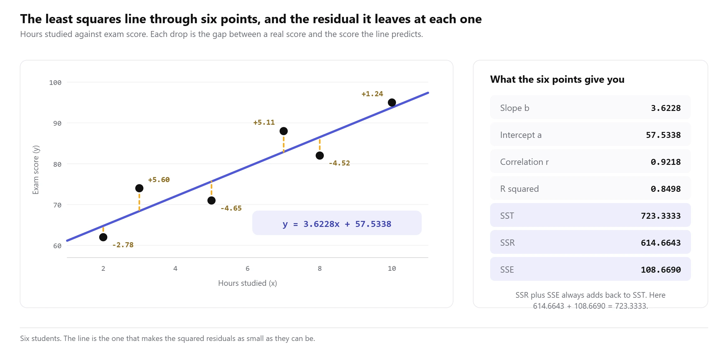
Six students recorded how many hours they studied and what they scored: 2 hours and 62 marks, 3 and 74, 5 and 71, 7 and 88, 8 and 82, 10 and 95.

Step 1, the two means. The hours add to 35, so x̄ = 35 ÷ 6 = 5.8333. The scores add to 472, so ȳ = 472 ÷ 6 = 78.6667.

Step 2, the two sums. For each student, multiply how far the hours sit from 5.8333 by how far the score sits from 78.6667, then add the six products: Σ(x − x̄)(y − ȳ) = 169.6667. Square the six hour distances and add those: Σ(x − x̄)² = 46.8333.

b = 169.6667 ÷ 46.8333 = 3.6228
a = 78.6667 − 3.6228 × 5.8333 = 57.5338
ŷ = 3.6228x + 57.5338

Read the slope in the units of the data: one more hour of study goes with about 3.62 more marks. The intercept of 57.53 is what the line predicts for zero hours, but nobody in this group studied for zero hours, so that number is an extrapolation and not a measurement.

Prediction is now arithmetic. A student who studies 9 hours: 3.6228 × 9 + 57.5338 = 90.1388, so roughly 90 marks. Nine sits inside the range 2 to 10 that the data covers, which is the only range the line has any authority over.

What r and R squared tell you

The correlation r runs from -1 to +1 and reports two things at once: which way the relationship goes, and how tightly the points hug a straight line. Our six points give r = 0.9218, so the relationship is positive and strong.

R squared is just r multiplied by itself, 0.8498 here, and it has a cleaner meaning. Start from how much the scores vary on their own, add up the squared gaps from the mean score, and you get SST = 723.3333. Of that, the line accounts for SSR = 614.6643 and leaves SSE = 108.6690 unexplained. Divide 614.6643 by 723.3333 and you have R squared. In plain terms, study hours account for 85% of the spread in these scores and something else accounts for the other 15%. The sum of squares calculator splits that three-way total on its own if you want to see it separately.

Two things R squared does not do. It cannot tell you that a straight line was the right shape, because a badly curved relationship can still return a high value. And it says nothing about cause. Ice cream sales and drowning deaths move together across the year with a respectable R squared, and neither one causes the other.

Residuals, and whether a straight line was the right shape

A residual is what the line got wrong at one point: the real y minus the predicted ŷ. Our six come out as -2.7794, +5.5979, -4.6477, +5.1068, -4.5160 and +1.2384.

Add them and you get exactly zero. That is true of every least squares line ever fitted, so it is a check on your arithmetic and nothing more. It is not evidence that the fit is any good.

The check that does mean something is the residual plot: residuals up the y axis, x along the bottom. If the straight line was the right shape, the residuals scatter in a flat band around zero with no pattern in them. If the real relationship curves, the line is forced to sit above the data at the ends and below it in the middle, and the residuals bend into a U that is obvious the moment you plot them.

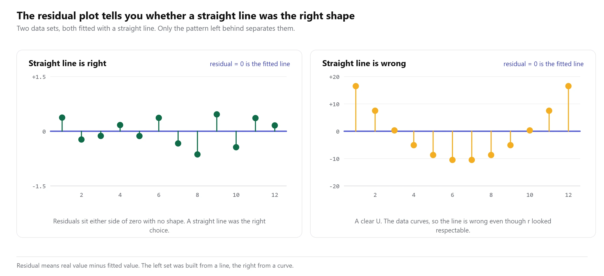
A fan shape is worth knowing too. If the residuals start small and spread out as x grows, the spread of y is not constant, and the p value and confidence interval further down this page stop being trustworthy even though the slope itself is still the least squares answer. A U rather than a fan is a different message: the straight line is the wrong shape entirely, and the fix is a curve. When y looks like it multiplies at each step rather than adding a fixed amount, the one to try is an exponential regression.

Look at the scatter plot before you trust the numbers

Frank Anscombe made this point better than anyone in Graphs in Statistical Analysis, published in The American Statistician in 1973. He built four sets of eleven points that share almost every summary number you would normally quote: the same mean of x, the same mean of y, the same regression line y = 3.00 + 0.50x, the same correlation of 0.816 and the same R squared of 0.67.

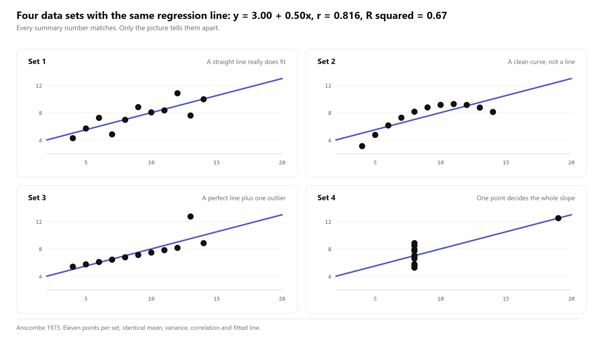
Only the first set is a case where the line is the right answer. The second is a smooth curve that a straight line has no business describing. The third is a perfect line with one point knocked out of place, and that single point drags the slope. In the fourth, ten of the eleven points sit at the same x value, so one far off point on its own decides the entire slope. A summary table cannot separate these four. A picture separates them instantly, which is why the calculator above draws the scatter plot before it prints anything else.

Is the slope real, or could it be chance?

Six students out of a whole class will give a slope of some sort even if hours and marks have nothing to do with each other. The question is whether 3.6228 is far enough from zero to take seriously.

Start with the typical size of a residual. Divide SSE by n − 2 and take the square root: √(108.6690 ÷ 4) = 5.2122 marks. Statistics calls that the standard error of the estimate, and it is a standard deviation of sorts, measured around the line instead of around the mean. Divide it by √46.8333 and you get 0.7616, the standard error of the slope.

t = 3.6228 ÷ 0.7616 = 4.7566 on 4 degrees of freedom
p = 0.0089
95% confidence interval for the slope: 1.5081 to 5.7374

A p value of 0.0089 sits below the usual 0.05 threshold, so the slope is distinguishable from zero. Now look at the confidence interval, because it is the more honest of the two. The data is consistent with anything from 1.5 to 5.7 extra marks per hour, a range wide enough that you could not plan around it. Six points buy you a direction and very little precision. Twenty points with the same underlying pattern would narrow that interval considerably.

Linear regression in Excel and Google Sheets

With hours in A2:A7 and scores in B2:B7, four formulas cover most homework and most reports:

• =SLOPE(B2:B7,A2:A7) returns 3.6228
• =INTERCEPT(B2:B7,A2:A7) returns 57.5338
• =RSQ(B2:B7,A2:A7) returns 0.8498, and =CORREL(A2:A7,B2:B7) returns 0.9218
• =FORECAST.LINEAR(9,B2:B7,A2:A7) returns 90.1388 without you having to build the equation first

Both spreadsheets want the y values before the x values in SLOPE, INTERCEPT, RSQ and FORECAST, which is the reverse of how everyone says it out loud. Swap them by accident and you will get a slope of 0.2346 instead of 3.6228, with no error message to warn you. CORREL is the exception and gives the same answer either way round.

For the standard errors, the t statistic and the sums of squares, =LINEST(B2:B7,A2:A7,TRUE,TRUE) returns a block five rows deep. The first row holds the slope and the intercept, the second holds their standard errors, the third holds R squared and the standard error of the estimate, and the last holds SSR and SSE. It is unlabelled, which is why most people give up on it.

Linear regression on a TI-84 or TI-83

1. Press STAT, choose 1: Edit, and type the x values into L1 and the y values into L2.
2. Turn the diagnostics on, or r and r squared will not appear. On newer operating systems press MODE, scroll to STAT DIAGNOSTICS and set it to ON. On older ones press 2nd then 0 for the catalog, scroll to DiagnosticOn and press ENTER twice.
3. Press STAT, move right to CALC, and choose 4: LinReg(ax+b). Press Calculate.
4. Read a = 3.6228 and b = 57.5338, with r squared = 0.8498 and r = 0.9218 underneath.

That third step is where marks get lost. In LinReg(ax+b) the calculator calls the slope a and the intercept b, which is the opposite of the a + bx convention almost every textbook uses. Option 8 on the same menu, LinReg(a+bx), matches the textbook and reports a as the intercept. Same line either way, so check which one you ran before you write the equation down.

Where regression questions go wrong

Putting the columns the wrong way round. Regressing y on x and regressing x on y give two different lines, not one line read two ways. They only coincide when r is exactly 1 or -1. Decide which variable you are predicting, and that one is y.

Rounding the slope before you use it. Round 3.6228 to 3.6 and the intercept becomes 57.6667 rather than 57.5338. The prediction at 9 hours shifts from 90.1388 to 90.0667. Small here, but the error grows with every step you take away from the mean, so carry four decimals through and round once at the end.

Predicting outside the data. Our line says a student studying 40 hours would score 202. The equation will happily produce that number. Nothing in the data supports it, and the relationship almost certainly flattens long before 40 hours.

Reading R squared as proof of cause. A high R squared says the line tracks the data. It does not rule out a third variable driving both columns, and it does not tell you which direction any causation runs in.

Deleting the point that spoils the fit. Set 3 of Anscombe’s quartet is one outlier away from a perfect straight line, and dropping it would push R squared close to 1. That is only legitimate if you can show the point was a recording error. An outlier you cannot explain is a finding, and it belongs in the write-up.