
Histogram maker
Paste your numbers and get a histogram you can download, plus the frequency table behind it and a read on the shape of the distribution.

 By Mohammad Majd · Reviewed by Susan Simmons✓ Fact-checked
How to use the histogram maker
- 1Paste your numbers
Commas, spaces or one per line all work, and so does a column copied straight out of Excel or Google Sheets.
- 2Press Make histogram
The bins are chosen for you with the Sturges rule, and the chart appears straight away.
- 3Tune it under the chart
Change the bin width, the start point or the number of bins, switch binning rule, pick a colour and add a title. The chart redraws as you go.
- 4Download it
Save the chart as a PNG for a report, or as an SVG if you want to edit it later. The table copies as text.
Chart title and axis labels
How these bins were worked out
What is a histogram?
A histogram splits a range of numbers into equal slices, called bins, and draws a bar for each one whose height is how many values landed inside it. The bars sit side by side with no gaps, because the bins cover a continuous range with nothing missing between them.
It answers a question a list of numbers cannot: where do the values pile up. Twenty exam marks between 58 and 97 tell you almost nothing as a list. Grouped into bins of 10, you can see at a glance whether most of the class sat in the 70s or whether the marks split into a strong group and a struggling one.
The bars only make sense if the bins are the same width. A bar twice as wide covering twice the range will look twice as important even when it is not, which is the one rule most hand-drawn histograms break.
How to make a histogram
Four steps, whether you are doing it by hand or checking what software gave you:
- Find the smallest and largest value. The distance between them is the range.
- Decide how many bins you want. Five to 15 is the usual band, and the rules below give you a starting number.
- Divide the range by the bin count to get a bin width, then round it to something readable such as 5 or 10.
- Count how many values fall in each bin and draw a bar that tall.
Worked example
Twenty heights in centimetres, from 158 up to 185. The range is 27.
Sturges suggests 6 bins for 20 values, and 27 divided by 6 is 4.5. Rounding the width up to 5 and starting at 155 gives six bins: 155 to 160, 160 to 165, and so on up to 185.
- 155 to 160: 1 value
- 160 to 165: 1
- 165 to 170: 4
- 170 to 175: 7
- 175 to 180: 4
- 180 to 185: 3
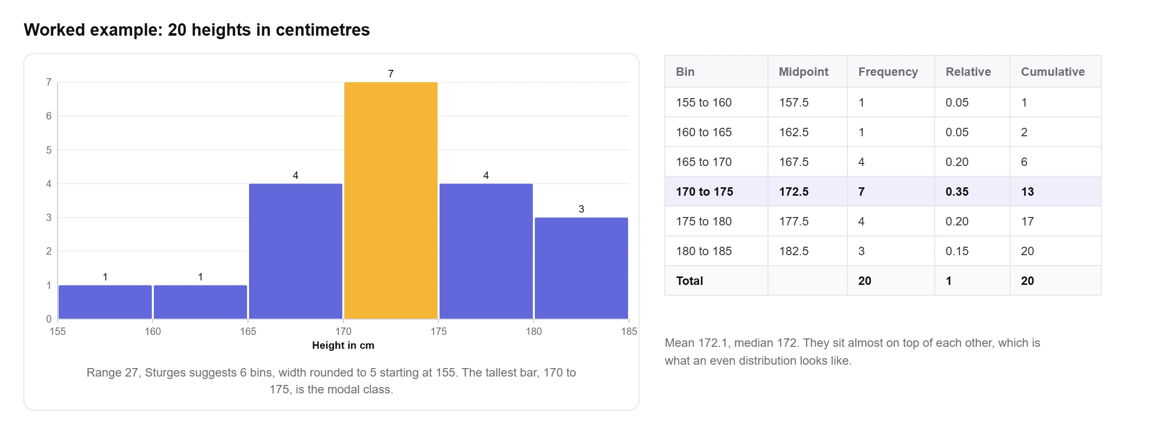
The counts add back to 20, which is the check worth doing every time. The tallest bar is 170 to 175, the mean is 172.1 and the median is 172. Mean and median sitting almost on top of each other, with the tall bar in the middle, is what an even distribution looks like. Click “Heights” in the calculator above to see it drawn.
How many bins should a histogram have?
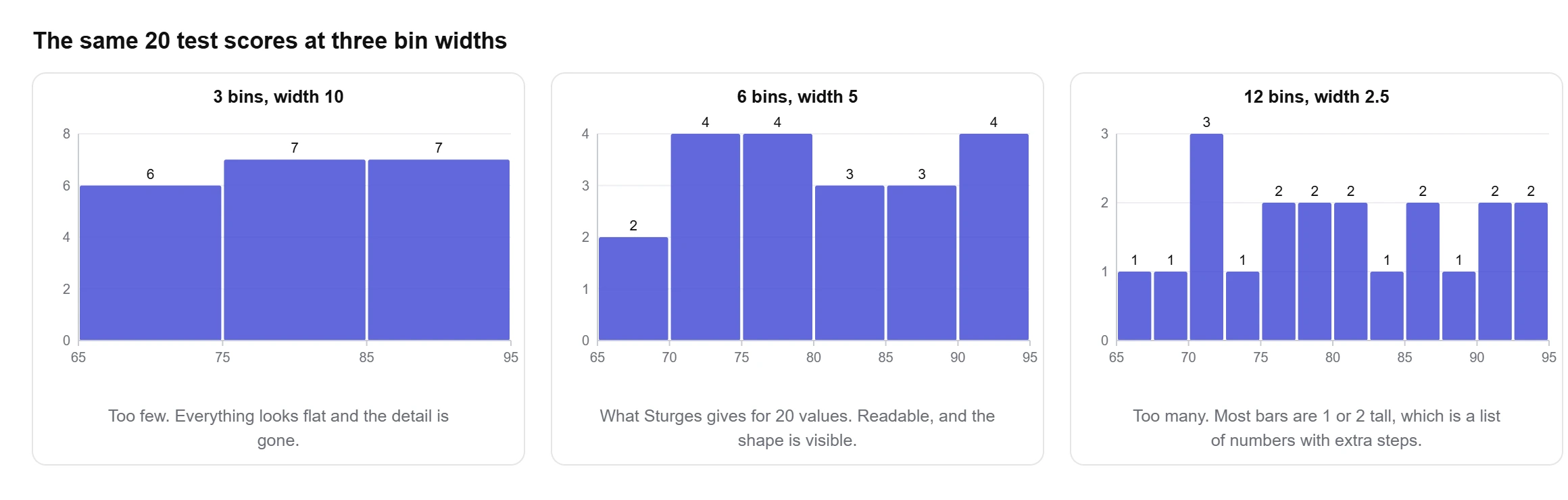
There is no correct answer, only answers that are easier or harder to read. Too few bins and two groups get merged into one bar. Too many and every bar is 1 or 2 values tall, which is a list of numbers with extra steps.
The OpenStax Statistics textbook puts the practical band at five to 15 bars for clarity, and suggests the square root of the number of values as a quick starting point. Four other rules are in common use, and the calculator lets you switch between all five:
| Rule | Formula | Bins for 20 values | Best for |
|---|---|---|---|
| Sturges | k = ⌈log₂ n⌉ + 1 | 6 | The common default. Fine up to a few hundred values. |
| Square root | k = ⌈√n⌉ | 5 | Quick mental arithmetic, and what many textbooks teach. |
| Rice | k = ⌈2 × n1/3⌉ | 6 | Larger data sets, where Sturges gives too few bins. |
| Scott | h = 3.49 × s × n−1/3 | 4 | Data that is roughly bell shaped. |
| Freedman-Diaconis | h = 2 × IQR × n−1/3 | 6 | Data with outliers, since the IQR ignores them. |
Scott and Freedman-Diaconis give you a bin width rather than a count, and the count falls out of dividing the range by that width. The 3.49 constant comes from David Scott’s 1979 Biometrika paper, which worked out the bin width that minimises error for normally distributed data. Both rules depend on spread, so they react to your standard deviation, and through it your variance, in a way the counting rules do not.
The honest way to use them is to try two or three and see whether the picture changes. If the shape survives Sturges, square root and Freedman-Diaconis, it is in the data. If it appears under one rule and vanishes under another, it was in the binning.
The frequency distribution table
Every histogram has a table underneath it, and for a lot of coursework the table is the part being marked. The calculator prints it with four columns beyond the bin itself.
- Frequency: how many values landed in the bin. These are the bar heights.
- Relative frequency: the count divided by the total. A bin holding 7 of 20 values has a relative frequency of 0.35.
- Cumulative frequency: a running total as you move up through the bins.
- Cumulative percent: the same running total as a percentage, which answers questions like what share of the class scored under 80.
A relative frequency histogram is the same chart with the y-axis switched from counts to proportions. The bars keep their shape and only the scale changes, which matters when you want to compare two groups of different sizes. Twelve out of 20 and sixty out of 100 are both 0.6, and only the relative version shows that. The Frequency, Relative and Percent buttons under the chart switch between the three.
What the shape of a histogram tells you
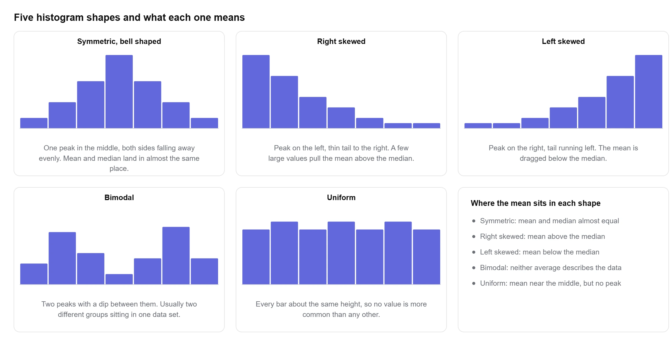
The outline of the bars is the reason to draw the thing. Five shapes cover most real data, and the calculator names the one it finds along with its reasoning. A histogram shows you that shape and a five number summary puts numbers on it, which is why the two are usually reported together.
Symmetric and bell shaped
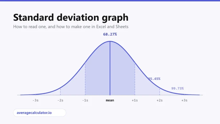
One peak near the middle with the bars falling away evenly on both sides. Mean and median land in nearly the same place. Heights, measurement errors and exam marks from a large group tend to look like this. Overlay a standard deviation graph on a histogram with this shape and the two line up closely.
Right skewed
The peak sits on the left and a thin tail stretches right. Salaries are the standard case: twenty salaries running from 22,000 to 240,000 have a mean of 57,300 and a median of only 34,000, because a handful of large values drag the mean up while leaving the median alone. Whenever the mean sits well above the median, expect a right skewed histogram, and read our note on mean vs median before reporting the average.
Left skewed
The mirror image. The peak is on the right and the tail runs left, which pulls the mean below the median. Test scores on an easy exam do this, since most people cluster near the top and a few low marks stretch the bottom.
Bimodal
Two separate peaks with a dip between them. This almost always means two different groups are sitting in one data set: two machines, two age groups, two shifts. The fix is to split the data and draw a histogram for each, because a single mean describing both peaks describes neither.
Uniform
Every bar is about the same height, so no value is more common than any other. Dice rolls and random numbers look like this, because every outcome is equally likely. With a small sample it is easy to see a flat histogram that is really just noise, so the calculator only calls a shape uniform when there are at least five values per bin to judge it on.
Histogram vs bar graph
They look similar and answer different questions. A histogram shows one numeric variable split into ranges. A bar graph compares separate categories.
- A histogram has no gaps between the bars, because the bins run into each other along a number line. A bar graph has gaps, because the categories are not next to anything.
- Histogram bars cannot be reordered. Moving the 70 to 80 bin next to the 90 to 100 bin would break the axis. Bar graph bars can be sorted any way you like.
- The x-axis of a histogram is numeric and continuous. The x-axis of a bar graph holds labels such as country, brand or colour.
- Bin width changes a histogram. Nothing equivalent exists for a bar graph, where one bar is one category, or for a pie chart, where one slice is one share of the total.
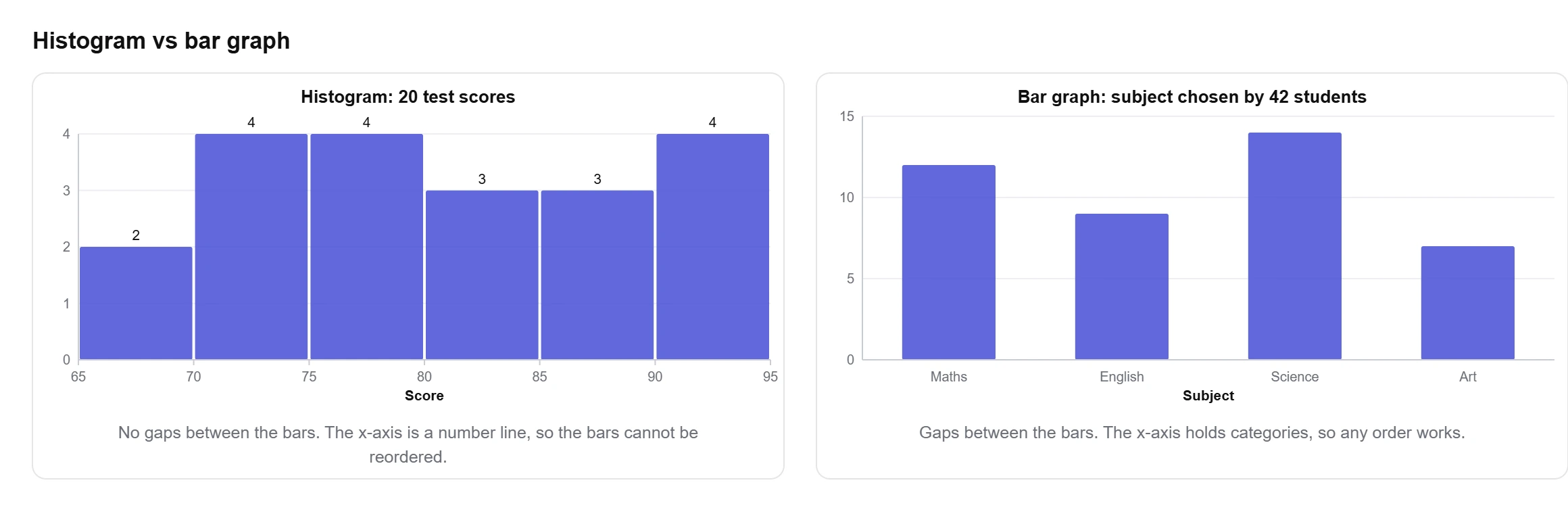
Sales by month is a bar graph, because months are categories. The distribution of order values is a histogram, because order value is a number that can land anywhere in a range.
Making a histogram in Excel and Google Sheets
Excel has had a built-in histogram chart since 2016. Select your column, open Insert, choose the statistic chart icon and pick Histogram. Excel chooses the bins for you, and you change them by right-clicking the x-axis, opening Format Axis and setting either the bin width or the number of bins.
Google Sheets does it through Insert, then Chart, then Chart type, then Histogram chart. Bin width sits under the Customise tab in the Histogram section. Sheets offers fewer bin widths than Excel does, which is worth knowing before you fight it.
Both of them hide the frequency table. If you need the counts written out, or you want to see what a different binning rule would do, paste the same column into the calculator above and you get the chart and the table together.
Why use this histogram maker?
What you get with this free histogram maker:
- The frequency distribution table printed under the chart, with relative frequency, cumulative frequency and cumulative percent.
- Five binning rules to switch between, or set the number of bins yourself.
- A plain-English read on the shape of your data, with the skewness and the peak count it was based on.
- Bin edges rounded to readable numbers such as 155 to 160, instead of 158 to 162.83.
- Download as PNG for a report, or as SVG if you want to edit the chart later.
- Grouped data input, so you can draw the chart straight from classes and counts you already have.
- Free to use
- No sign-up
- PNG and SVG download
- Frequency table included
- 5 binning rules
Frequently asked questions
How do I make my own histogram?
Paste your numbers into the box above and press Make histogram. The calculator picks the bins, counts the values in each one and draws the chart, and you can change the binning rule or set the bin count yourself.
What is the difference between a histogram and a bar graph?
A histogram shows one numeric variable split into ranges and has no gaps between the bars. A bar graph compares separate categories and has gaps. Histogram bars cannot be reordered; bar graph bars can.
How many bins should I use?
Five to 15 covers most data. Sturges gives 6 bins for 20 values and 8 for 100. If two rules disagree, try both and keep the one where the shape is clearest.
What does a right skewed histogram mean?
The bars peak on the left and trail off to the right, which happens when a few large values stretch the top end. The mean ends up above the median, so the median usually describes the data better.
What does a bimodal histogram mean?
Two clear peaks with a dip between them, which normally means two groups are mixed in one data set. Splitting the data and charting each group separately is the usual fix.
Can I download the histogram?
Yes. The PNG button saves an image at twice the display size for reports and slides, and the SVG button saves a vector file you can edit in any design tool.
What software is best for creating histograms?
For a quick chart, an online tool is fastest because there is nothing to install. Excel and Google Sheets both have a histogram chart type if the data already lives in a spreadsheet, and R or Python suit you if the chart is part of a longer analysis.
Can I create a histogram in Word?
Word has no histogram chart type of its own. Insert a chart, which opens a small Excel sheet, and pick Histogram from the statistic charts there. Making the chart elsewhere and pasting the image in is usually quicker.
Explore our other calculators
 Average calculator
 Average percentage calculator
 Average time calculator
 Degrees of freedom calculator
 Exponential Regression Calculator
 Five Number Summary Calculator
 IQR calculator
 Linear regression calculator
 Mean, Median, Mode and Range Calculator
 Outlier Calculator
 Pie Chart Maker
 Probability Calculator
 Standard deviation calculator
 Sum of Squares Calculator
 Variance calculator
 Weighted average calculator
Our latest blogs
Four quartile methods, one data set, three answers for Q1
Standard deviation graph: how to read one and how to make one
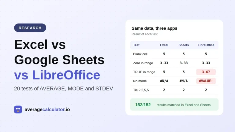
Excel vs Google Sheets vs LibreOffice: how average functions handle blanks, zeros and text
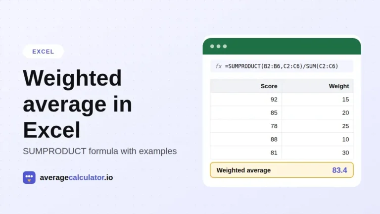
How to calculate a weighted average in Excel, with examples
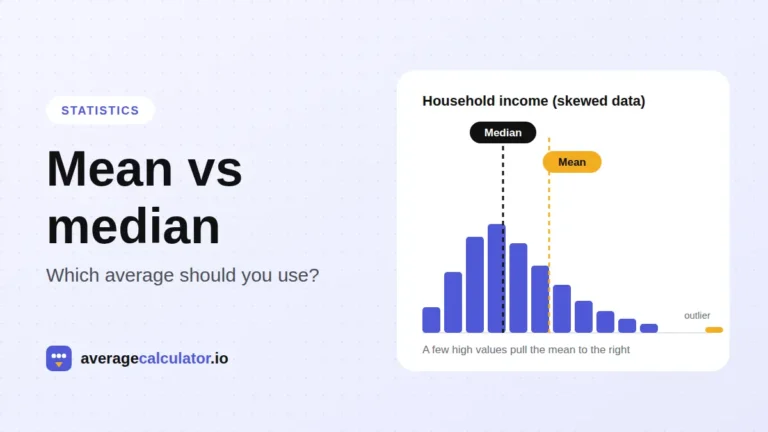
Mean vs median: which average should you use?
Who made this calculator
Spotted a mistake in this calculator? Tell us the numbers you used and what you expected, and we will check it.
Report an error